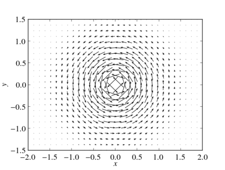
A vector field assigns to every point in space some vector. Vector fields are used in many branches of physics, e.g., to describe force fields, electromagnetic fields or velocity fields. Two-dimensional vector fields can be easily visualized using Python and the popular matplotlib package. As an example let us visualize the vector field
\begin{equation}
\vec E(\vec r) =
\begin{pmatrix}
E_x(x, y) \\ E_y(x, y)
\end{pmatrix} =
\begin{pmatrix}
-y\frac{\exp(-(x^2+y^2))}{\sqrt{x^2+y^2}} \\
x\frac{\exp(-(x^2+y^2))}{\sqrt{x^2+y^2}}
\end{pmatrix}\,.
\end{equation}Using the quiver function this is not difficult as the following example shows.
#!/usr/bin/env python

# import useful modules
import matplotlib
from numpy import *
from pylab import *

# use LaTeX, choose nice some looking fonts and tweak some settings
matplotlib.rc('font', family='serif')
matplotlib.rc('font', size=16)
matplotlib.rc('legend', fontsize=16)
matplotlib.rc('legend', numpoints=1)
matplotlib.rc('legend', handlelength=1.5)
matplotlib.rc('legend', frameon=False)
matplotlib.rc('xtick.major', pad=7)
matplotlib.rc('xtick.minor', pad=7)
matplotlib.rc('text', usetex=True)
matplotlib.rc('text.latex',
              preamble=[r'\usepackage[T1]{fontenc}',
                        r'\usepackage{amsmath}',
                        r'\usepackage{txfonts}',
                        r'\usepackage{textcomp}'])

close('all')
figure(figsize=(6, 4.5))

# generate grid
x=linspace(-2, 2, 32)
y=linspace(-1.5, 1.5, 24)
x, y=meshgrid(x, y)
# calculate vector field
vx=-y/sqrt(x**2+y**2)*exp(-(x**2+y**2))
vy= x/sqrt(x**2+y**2)*exp(-(x**2+y**2))
# plot vecor field
quiver(x, y, vx, vy, pivot='middle', headwidth=4, headlength=6)
xlabel('$x$')
ylabel('$y$')
axis('image')
show()
savefig('visualization_vector_fields_1.png')
In a second example we will try to visualize the vector field of an electric dipole consisting of a positive charge $q$ at $\vec r_+$ and a negative charge $-q$ at $\vec r_-$. Its electromagnetic field is given by
\begin{equation}
\vec E(\vec r) = \frac{q}{4\pi\varepsilon_0}\left(
\frac{\vec r-\vec r_+}{|\vec r-\vec r_+|^3} – \frac{\vec r-\vec r_-}{|\vec r-\vec r_-|^3}
\right)
\end{equation}and we will plot its vector field in the $x$-$y$-plane. Similarly to our first example the Python code is given as follows.
#!/usr/bin/env python

# import useful modules
import matplotlib
from numpy import *
from pylab import *

# use LaTeX, choose nice some looking fonts and tweak some settings
matplotlib.rc('font', family='serif')
matplotlib.rc('font', size=16)
matplotlib.rc('legend', fontsize=16)
matplotlib.rc('legend', numpoints=1)
matplotlib.rc('legend', handlelength=1.5)
matplotlib.rc('legend', frameon=False)
matplotlib.rc('xtick.major', pad=7)
matplotlib.rc('xtick.minor', pad=7)
matplotlib.rc('text', usetex=True)
matplotlib.rc('text.latex',
              preamble=[r'\usepackage[T1]{fontenc}',
                        r'\usepackage{amsmath}',
                        r'\usepackage{txfonts}',
                        r'\usepackage{textcomp}'])

close('all')
figure(figsize=(6, 4.5))

# generate grid
x=linspace(-2, 2, 32)
y=linspace(-1.5, 1.5, 24)
x, y=meshgrid(x, y)

def E(q, a, x, y):
    return q*(x-a[0])/((x-a[0])**2+(y-a[1])**2)**(1.5), \
        q*(y-a[1])/((x-a[0])**2+(y-a[1])**2)**(1.5)

# calculate vector field
Ex1, Ey1=E(1, [-1, 0], x, y)
Ex2, Ey2=E(-1, [1, 0], x, y)
Ex=Ex1+Ex2
Ey=Ey1+Ey2
# plot vecor field
quiver(x, y, Ex, Ey, pivot='middle', headwidth=4, headlength=6)
xlabel('$x$')
ylabel('$y$')
axis('image')
show()
savefig('visualization_vector_fields_2.png')
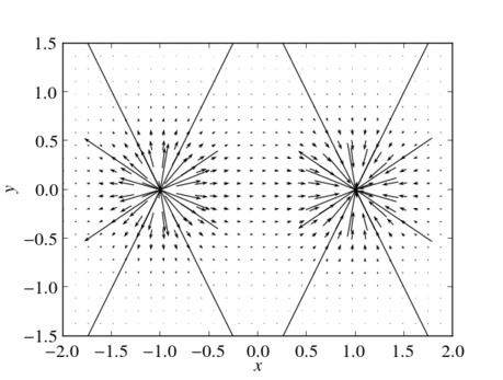
The dipole’s vector field has singularities at $r_+$ and $r_-$ where the length of the vectors to plot dives. Consequently the plot above looks not very eye candy. One possible measure to avoid vectors of diverging length is to normalize the all vectors to unity as shown below.
#!/usr/bin/env python

# import usefull modules
import matplotlib
from numpy import *
from pylab import *

# use LaTeX, choose nice some looking fonts and tweak some settings
matplotlib.rc('font', family='serif')
matplotlib.rc('font', size=16)
matplotlib.rc('legend', fontsize=16)
matplotlib.rc('legend', numpoints=1)
matplotlib.rc('legend', handlelength=1.5)
matplotlib.rc('legend', frameon=False)
matplotlib.rc('xtick.major', pad=7)
matplotlib.rc('xtick.minor', pad=7)
matplotlib.rc('text', usetex=True)
matplotlib.rc('text.latex',
              preamble=[r'\usepackage[T1]{fontenc}',
                        r'\usepackage{amsmath}',
                        r'\usepackage{txfonts}',
                        r'\usepackage{textcomp}'])

close('all')
figure(figsize=(6, 4.5))

# generate grid
x=linspace(-2, 2, 32)
y=linspace(-1.5, 1.5, 24)
x, y=meshgrid(x, y)

def E(q, a, x, y):
    return q*(x-a[0])/((x-a[0])**2+(y-a[1])**2)**(1.5), \
        q*(y-a[1])/((x-a[0])**2+(y-a[1])**2)**(1.5)

# calculate vector field
Ex1, Ey1=E(1, [-1, 0], x, y)
Ex2, Ey2=E(-1, [1, 0], x, y)
Ex=Ex1+Ex2
Ey=Ey1+Ey2
# plot normalized vecor field
quiver(x, y, Ex/sqrt(Ex**2+Ey**2), Ey/sqrt(Ex**2+Ey**2), pivot='middle', headwidth=4, headlength=6)
xlabel('$x$')
ylabel('$y$')
axis('image')
show()
savefig('visualization_vector_fields_3.png')
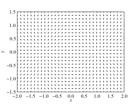
The vector field of an electric dipole in the $x$-$y$-plane with $r_+=(-1,0,0)$ and $r_-=(1,0,0)$. All vectors normalized to unity. Thus, the plot visualizes the direction of the electric dipole field, but not the field strength.
Normalizing the vector field to unity has the drawback of loosing information about the field strength. An alternative approach to get rid of extremely long vectors is to plot only those vectors whose lengths is below some given threshold $E_{\mathrm{max}}$. This can be archived by replacing vectors which are too long by some invalid value, that is by the value nan (not a number).
#!/usr/bin/env python

# import useful modules
import matplotlib
from numpy import *
from pylab import *

# use LaTeX, choose nice some looking fonts and tweak some settings
matplotlib.rc('font', family='serif')
matplotlib.rc('font', size=16)
matplotlib.rc('legend', fontsize=16)
matplotlib.rc('legend', numpoints=1)
matplotlib.rc('legend', handlelength=1.5)
matplotlib.rc('legend', frameon=False)
matplotlib.rc('xtick.major', pad=7)
matplotlib.rc('xtick.minor', pad=7)
matplotlib.rc('text', usetex=True)
matplotlib.rc('text.latex',
              preamble=[r'\usepackage[T1]{fontenc}',
                        r'\usepackage{amsmath}',
                        r'\usepackage{txfonts}',
                        r'\usepackage{textcomp}'])

close('all')
figure(figsize=(6, 4.5))

# generate grid
x=linspace(-2, 2, 32)
y=linspace(-1.5, 1.5, 24)
x, y=meshgrid(x, y)

def E(q, a, x, y):
    return q*(x-a[0])/((x-a[0])**2+(y-a[1])**2)**(1.5), \
        q*(y-a[1])/((x-a[0])**2+(y-a[1])**2)**(1.5)

# calculate vector field
Ex1, Ey1=E(1, [-1, 0], x, y)
Ex2, Ey2=E(-1, [1, 0], x, y)
Ex=Ex1+Ex2
Ey=Ey1+Ey2
# remove vector with length larger than E_max
E_max=10
E=sqrt(Ex**2+Ey**2)
k=find(E.flat[:]>E_max)
Ex.flat[k]=nan
Ey.flat[k]=nan
# plot vecor field
quiver(x, y, Ex, Ey, pivot='middle', headwidth=4, headlength=6)
xlabel('$x$')
ylabel('$y$')
axis('image')
show()
savefig('visualization_vector_fields_4.png')
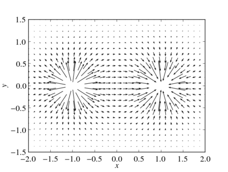
The vector field of an electric dipole in the $x$-$y$-plane with $r_+=(-1,0,0)$ and $r_-=(1,0,0)$. All vectors longer than some threshold are removed from the plot. Thus, the plot visualizes both the direction and the strength of the electric dipole field while avoiding vectors of extreme length.