Finding the eigenvalues and eigenvectors of large hermitian matrices is a key problem of (numerical) quantum mechanics. Often, however, the matrices of interest are much too large to employ exact methods. A popular and powerful approximation method is based on the Lanczos algorithm. The Lanczos algorithm determines an orthonormal basis of the Kyrlov sub-space $\mathcal{K}_k(\Psi, \hat H)$. The Kyrlov sub-space $\mathcal{K}_k(\Psi, \hat H)$ is the linear space that is spanned by the vectors $\Psi$, $\hat H\Psi$, ${\hat H}^2\Psi$, …, ${\hat H}^{k-1}\Psi$ with $k\le \dim\hat H$. Furthermore, the Lanczos algorithm constructs a real symmetric tridiagonal matrix $\hat H’$ with $\dim\hat H’=k$ that is an approximation of $\hat H$ in the sense that the eigenvalues of $\hat H’$ are close to some eigenvalues of $\hat H$. The eigenvectors of $\hat H$ can be approximated via the eigenvectors of $\hat H’$. Thus, the Lanczos algorithm reduces the problem of matrix diagonalization of large hermitian matrices to the diagonalization of a (usually) much smaller real symmetric tridiagonal matrix, which is a much simpler task.
The Lanczos algorithm has been applied to many problems of nonrelativistic quantum mechanics, in particular bound state calculations and time propagation. In a recent work (arXiv:1407.7370) we evaluated the Lanczos algorithm for solving the time-independent as well as the time-dependent relativistic Dirac equation with arbitrary electromagnetic fields. We demonstrate that the Lanczos algorithm can yield very precise eigenenergies and allows very precise time propagation of relativistic wave packets. The Dirac Hamiltonian’s property of not being bounded does not hinder the applicability of the Lanczos algorithm. As the Lanczos algorithm requires only matrix-vector and inner products, which both can be efficiently parallelized, it is an ideal method for large-scale calculations. The excellent parallelization capabilities are demonstrated by a parallel implementation of the Dirac Lanczos propagator utilizing the Message Passing Interface standard.
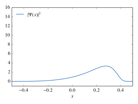
The following python code shows how to solve the time-dependent free one-dimensional Dirac equation via the Lanczos algorithm. The Hamiltonian
\begin{equation}
\hat H = c \begin{pmatrix}
0 & 1 \\ 1 & 0
\end{pmatrix} \left(-\mathrm{i}\frac{\partial}{\partial x} \right) + \begin{pmatrix}
1 & 0 \\ 0 & -1
\end{pmatrix}m_0c^2
\end{equation}is approximated via second order finite differences. A detailed description of the Lanczos algorithm and its application to the Dirac equation is given in arXiv:1407.7370.
#!/usr/bin/env python
# -*- coding: utf-8 -*-

# import useful modules
import matplotlib
from math import factorial
from numpy import *
from pylab import *
from numpy.polynomial.hermite import *

# use LaTeX, choose some nice looking fonts and tweak some settings
matplotlib.rc('font', family='serif')
matplotlib.rc('font', size=16)
matplotlib.rc('legend', fontsize=16)
matplotlib.rc('legend', numpoints=1)
matplotlib.rc('legend', handlelength=1.5)
matplotlib.rc('legend', frameon=False)
matplotlib.rc('xtick.major', pad=7)
matplotlib.rc('xtick.minor', pad=7)
matplotlib.rc('lines', lw=1.5)
matplotlib.rc('text', usetex=True)
matplotlib.rc('text.latex',
              preamble=[r'\usepackage[T1]{fontenc}',
                        r'\usepackage{amsmath}',
                        r'\usepackage{txfonts}',
                        r'\usepackage{textcomp}'])

close('all')
figure(figsize=(6, 4.5))

c=137.0359998  # speed of light in a.u.
N=1024+512

# the 1d Dirac Hamiltonian
def H(Psi, x, t, dt):
    Psi=reshape(Psi, (N, 2))
    dx=x[1]-x[0]
    Psi_new=empty_like(Psi)
    Psi_new[1:-1, 0]=-1j*c*(Psi[2:, 1]-Psi[0:-2, 1])/(2*dx) + c**2*Psi[1:-1, 0]
    Psi_new[1:-1, 1]=-1j*c*(Psi[2:, 0]-Psi[0:-2, 0])/(2*dx) - c**2*Psi[1:-1, 1]
    Psi_new[0, 0]=Psi_new[0, 1]=0
    Psi_new[-1, 0]=Psi_new[-1, 1]=0
    Psi_new*=dt
    return reshape(Psi_new, 2*N)

# the Lanczos algorithm
def Lanczos(Psi, x, t, dt, H, m):
    Psi_=Psi.copy()
    # run Lanczos algorithm to calculate basis of Krylov space
    V_j, V_j_1=[], []
    A=zeros((m, m))
    norms=zeros(m)
    for j in range(0, m):
        norms[j]=norm(Psi_)
        V_j=Psi_/norms[j]
        Psi_=H(V_j, x, t, dt)
        if j>0:
            A[j-1, j]=A[j, j-1]=vdot(V_j_1, Psi_).real
            Psi_-=A[j-1, j]*V_j_1
        A[j, j]=vdot(V_j, Psi_).real
        Psi_-=A[j, j]*V_j
        V_j_1, V_j=V_j, V_j_1
    # diagonalize A
    l, v=eig(A)
    # calculate matrix exponential in Krylov space
    c=dot(v, dot(diag(exp(-1j*l)), v[0, :]*norms[0]))
    # run Lanczos algorithm 2nd time to transform result into original space
    Psi_, Psi=Psi, zeros_like(Psi)
    for j in range(0, m):
        V_j=Psi_/norms[j]
        Psi+=c[j]*V_j
        Psi_=H(V_j, x, t, dt)
        if j>0:
            A[j-1, j]=A[j, j-1]=vdot(V_j_1, Psi_).real
            Psi_-=A[j-1, j]*V_j_1
        A[j, j]=vdot(V_j, Psi_).real
        Psi_-=A[j, j]*V_j
        V_j_1, V_j=V_j, V_j_1
    return Psi

# define computational grid
x0, x1=-0.5, 0.5
x=linspace(x0, x1, N)
dx=x[1]-x[0]       # size of spatial grid spacing
dt=4./c**2         # temporal step size

# constuct momentum grid
dp=2*pi/(N*dx)
p=(arange(0, N)-0.5*(N-1))*dp
# choose initial condition
p_mu=75.       # mean momentum
sigma_p=50.    # momentum width
x_mu=-0.05     # mean position
# upper and lower components of free particle states,
# see e.g. Thaller »Advanced visual quantum mechanics«
d_p=sqrt(0.5+0.5/sqrt(1+p**2/c**2))
d_m=sqrt(0.5-0.5/sqrt(1+p**2/c**2))
d_m[p<0]*=-1
# initial condition in momentum space,
# gaussian wave packet of positive energy states
rho=(2*pi*sigma_p**2)**(-0.25)*exp(-(p-p_mu)**2/(4*sigma_p**2) - 1j*p*x_mu)
Psi=zeros((N, 2), dtype='complex')
Psi[:, 0]=d_p*rho
Psi[:, 1]=d_m*rho
# transform into real space with correct complex phases
Psi[:, 0]*=exp(1j*x[0]*dp*arange(0, N))
Psi[:, 1]*=exp(1j*x[0]*dp*arange(0, N))
Psi=ifft(Psi, axis=0)
Psi[:, 0]*=dp*N/sqrt(2*pi)*exp(1j*x*p[0])
Psi[:, 1]*=dp*N/sqrt(2*pi)*exp(1j*x*p[0])

# propagate
for k in range(0, 20):
    # plot wave function
    clf()
    plot(x, Psi[:, 0].real**2+Psi[:, 0].imag**2+
         Psi[:, 1].real**2+Psi[:, 1].imag**2,
         color='#266bbd', label=r'$|\Psi(x)|^2'$)
    gca().set_xlim(x0, x1)
    gca().set_ylim(-1, 16)
    xlabel(r'$x)
    legend(loc='upper left')
    tight_layout()
    draw()
    show()
    pause(0.05)
    Psi=reshape(Lanczos(reshape(Psi, 2*N), x, 0, dt, H, 128), (N, 2)